3. Feature Reduction
Once a meaningful set of time series features has been extracted for each variable and participant, the total number of data points sometimes remains too large for the desired clustering algorithm (Altman & Krzywinski, 2018). In such cases, it is often recommended to perform an (optional) feature reduction. The commmonly used feature reduction procedures can commonly be separated into feature selection and feature projection. We provide a more detailed discussion of the pros and cons of the different approaches. For this illustration we focus on feature projections, which have been popular because they are efficient, widely available, and applicable to a wide range of data types. That being said, because feature selection procedures have the benefit that they retain the interpretable feature labels directly and immediately indicate which features were most informative in the sample (Carreira-Perpiñán, 1997), we recommend users to carefully consider the most useful option for their use case.
It is important to note again that a feature reduction step is not always necessary. Especially methods such as k-means are well equipped to deal with relatively large data sets (Jain, 2010). It is important to check whether the full feature set leads to convergence issues or unstable cluster solutions. We go through the feature reduction steps as an exemplary illustration only.
Principal Component Analysis
We, specifically, selected the commonly used principal component analysis (PCA). PCAs have the distinct benefit that they are well-established within the psychometric literature (Jolliffe, 2011) and can broadly be applied to a wide variety of studies in an automatized manner (Abdi & Williams, 2010). As our aim is to present a general illustration that can also be adopted across use cases, we present the workflow using a PCA here but we encourage users to consider more specialized methods as well.
Running the PCA
To use the PCA with our extracted time series features, we focus on a transformed feature set where the features are standardized across participants to ensure that all features are weighted equally. This transformation was already calculated as part of the featureExtractor() function and we now save it as a data frame scaled_data.
We then enter the standardized features into the principal component analysis using the prcomp() function from the stats package (R Core Team, 2024).
res.pca <- prcomp(scaled_data, scale. = FALSE)
pca_summary <- summary(res.pca)

# extract explained variances
res.varExplained <- data.frame(
  Explained_Variance = cumsum(summary(res.pca)[["importance"]]['Proportion of Variance',]),
  Components = seq(1, length(cumsum(summary(res.pca)[["importance"]]['Proportion of Variance',])), 1)
)
The PCA uses linear transformations in such a way that the first component captures the most possible variance of the original data (e.g., by finding a vector that maximizes the sum of squared distances; see Jolliffe (2002), Abdi & Williams (2010)). The following components will then use the same method to iteratively explain the most of the remaining variance while also ensuring that the components are linearly uncorrelated (Shlens, 2014). In practice, this meant that the PCA decomposed the 72 features into 72 principal components but now (because of the uncorrelated linear transformations) the first few principal components will capture a majority of the variance (see Table 1).
# Creating a data frame to hold variance details
variance_df <- data.frame(
  Component = 1:length(pca_summary$sdev),
  `Standard Deviation` = pca_summary$sdev,
  `Proportion of Variance` = pca_summary$importance[2, ],
  `Cumulative Proportion` = pca_summary$importance[3, ]
)

# Producing the kable output
variance_df %>%
 kbl(.,
      escape = FALSE,
      booktabs = TRUE,
      label = "pca_summary",
      format = "html",
      digits = 2,
      linesep = "",
      col.names = c("Component", "Standard Deviation", "Proportion of Variance", "Cumulative Proportion"),
      caption = "PCA Component Summary") %>%
  kable_classic(
    full_width = FALSE,
    lightable_options = "hover",
    html_font = "Cambria"
  ) %>%
scroll_box(width = "100%", height = "500px")| Component | Standard Deviation | Proportion of Variance | Cumulative Proportion | |
|---|---|---|---|---|
| PC1 | 1 | 2.75 | 0.11 | 0.11 |
| PC2 | 2 | 2.51 | 0.09 | 0.19 |
| PC3 | 3 | 1.97 | 0.05 | 0.25 |
| PC4 | 4 | 1.90 | 0.05 | 0.30 |
| PC5 | 5 | 1.73 | 0.04 | 0.34 |
| PC6 | 6 | 1.67 | 0.04 | 0.38 |
| PC7 | 7 | 1.59 | 0.04 | 0.41 |
| PC8 | 8 | 1.49 | 0.03 | 0.44 |
| PC9 | 9 | 1.46 | 0.03 | 0.47 |
| PC10 | 10 | 1.38 | 0.03 | 0.50 |
| PC11 | 11 | 1.35 | 0.03 | 0.52 |
| PC12 | 12 | 1.32 | 0.02 | 0.55 |
| PC13 | 13 | 1.30 | 0.02 | 0.57 |
| PC14 | 14 | 1.28 | 0.02 | 0.59 |
| PC15 | 15 | 1.24 | 0.02 | 0.62 |
| PC16 | 16 | 1.20 | 0.02 | 0.64 |
| PC17 | 17 | 1.17 | 0.02 | 0.65 |
| PC18 | 18 | 1.15 | 0.02 | 0.67 |
| PC19 | 19 | 1.13 | 0.02 | 0.69 |
| PC20 | 20 | 1.07 | 0.02 | 0.71 |
| PC21 | 21 | 1.06 | 0.02 | 0.72 |
| PC22 | 22 | 1.03 | 0.01 | 0.74 |
| PC23 | 23 | 1.00 | 0.01 | 0.75 |
| PC24 | 24 | 0.99 | 0.01 | 0.76 |
| PC25 | 25 | 0.96 | 0.01 | 0.78 |
| PC26 | 26 | 0.94 | 0.01 | 0.79 |
| PC27 | 27 | 0.93 | 0.01 | 0.80 |
| PC28 | 28 | 0.89 | 0.01 | 0.81 |
| PC29 | 29 | 0.88 | 0.01 | 0.82 |
| PC30 | 30 | 0.86 | 0.01 | 0.83 |
| PC31 | 31 | 0.84 | 0.01 | 0.84 |
| PC32 | 32 | 0.83 | 0.01 | 0.85 |
| PC33 | 33 | 0.81 | 0.01 | 0.86 |
| PC34 | 34 | 0.79 | 0.01 | 0.87 |
| PC35 | 35 | 0.77 | 0.01 | 0.88 |
| PC36 | 36 | 0.75 | 0.01 | 0.89 |
| PC37 | 37 | 0.73 | 0.01 | 0.89 |
| PC38 | 38 | 0.72 | 0.01 | 0.90 |
| PC39 | 39 | 0.69 | 0.01 | 0.91 |
| PC40 | 40 | 0.67 | 0.01 | 0.91 |
| PC41 | 41 | 0.64 | 0.01 | 0.92 |
| PC42 | 42 | 0.64 | 0.01 | 0.93 |
| PC43 | 43 | 0.61 | 0.01 | 0.93 |
| PC44 | 44 | 0.60 | 0.01 | 0.94 |
| PC45 | 45 | 0.59 | 0.00 | 0.94 |
| PC46 | 46 | 0.58 | 0.00 | 0.94 |
| PC47 | 47 | 0.56 | 0.00 | 0.95 |
| PC48 | 48 | 0.54 | 0.00 | 0.95 |
| PC49 | 49 | 0.53 | 0.00 | 0.96 |
| PC50 | 50 | 0.51 | 0.00 | 0.96 |
| PC51 | 51 | 0.50 | 0.00 | 0.96 |
| PC52 | 52 | 0.48 | 0.00 | 0.97 |
| PC53 | 53 | 0.47 | 0.00 | 0.97 |
| PC54 | 54 | 0.44 | 0.00 | 0.97 |
| PC55 | 55 | 0.44 | 0.00 | 0.98 |
| PC56 | 56 | 0.42 | 0.00 | 0.98 |
| PC57 | 57 | 0.41 | 0.00 | 0.98 |
| PC58 | 58 | 0.40 | 0.00 | 0.98 |
| PC59 | 59 | 0.39 | 0.00 | 0.98 |
| PC60 | 60 | 0.37 | 0.00 | 0.99 |
| PC61 | 61 | 0.36 | 0.00 | 0.99 |
| PC62 | 62 | 0.35 | 0.00 | 0.99 |
| PC63 | 63 | 0.34 | 0.00 | 0.99 |
| PC64 | 64 | 0.31 | 0.00 | 0.99 |
| PC65 | 65 | 0.29 | 0.00 | 0.99 |
| PC66 | 66 | 0.28 | 0.00 | 1.00 |
| PC67 | 67 | 0.27 | 0.00 | 1.00 |
| PC68 | 68 | 0.25 | 0.00 | 1.00 |
| PC69 | 69 | 0.23 | 0.00 | 1.00 |
| PC70 | 70 | 0.23 | 0.00 | 1.00 |
| PC71 | 71 | 0.20 | 0.00 | 1.00 |
| PC72 | 72 | 0.17 | 0.00 | 1.00 |
Component Selection
We can then decide how much information (i.e., variance) we are willing to sacrifice for a reduced dimensionality. A common rule of thumb is to use the principal components that jointly explain 70–90% of the original variance (Jackson, 2003). For our illustration, we chose a 80% of the cumulative percentage explained variance as the cutoff (i.e., cutoff_percentage)
This means that we select the first 27 principal components that explain 80% of the variance in the original 72 features (reducing the dimensionality by 62.50%).
fviz_eig(res.pca,
         addlabels = TRUE,
         choice = "variance",
         ncp = pca_cutoff,
         barfill = "#a6a6a6",
         barcolor = "transparent",
         main = "Scree Plot of Explained Variance per Principal Component",
         xlab = "Principal Components") +
         theme_Publication() +
  theme(text = element_text(size = 14, color = "#333333"),
        axis.title = element_text(size = 16, face = "bold", color = "#555555"),
        plot.title = element_text(size = 18, hjust = 0.5, face = "bold", color = "#444444"),
        legend.position = "none",
        panel.grid.minor = element_blank())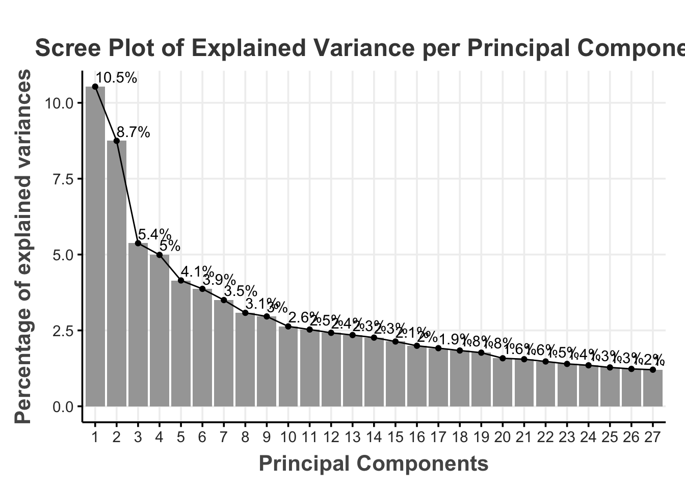
res.varExplained <- data.frame(
  Explained_Variance = cumsum(summary(res.pca)[["importance"]]['Proportion of Variance',]),
  Components = seq(1, length(cumsum(summary(res.pca)[["importance"]]['Proportion of Variance',])), 1)
)

ggplot(data = res.varExplained, aes(x = Components, y = Explained_Variance)) +
  geom_point() +
  geom_line() +
  geom_vline(mapping = aes(xintercept = pca_cutoff), linetype = "longdash") +
  geom_hline(mapping = aes(yintercept = cutoff_percentage), linetype = "longdash") +
  geom_text(aes(x = pca_cutoff, y = min(Explained_Variance) + 0.01),
            label = paste0(pca_cutoff, " components"), hjust = -0.1, vjust = 0, size = 3) +
  geom_text(aes(x = min(Components), y = cutoff_percentage),
            label = paste0(cutoff_percentage*100, "%"), hjust = 0, vjust = -1, size = 3) +
  labs(title = "Cumulative Proportion of Variance Explained",
       x = "Number of Components",
       y = "Proportion of Variance Explained") +
  tsFeatureExtracR::theme_Publication()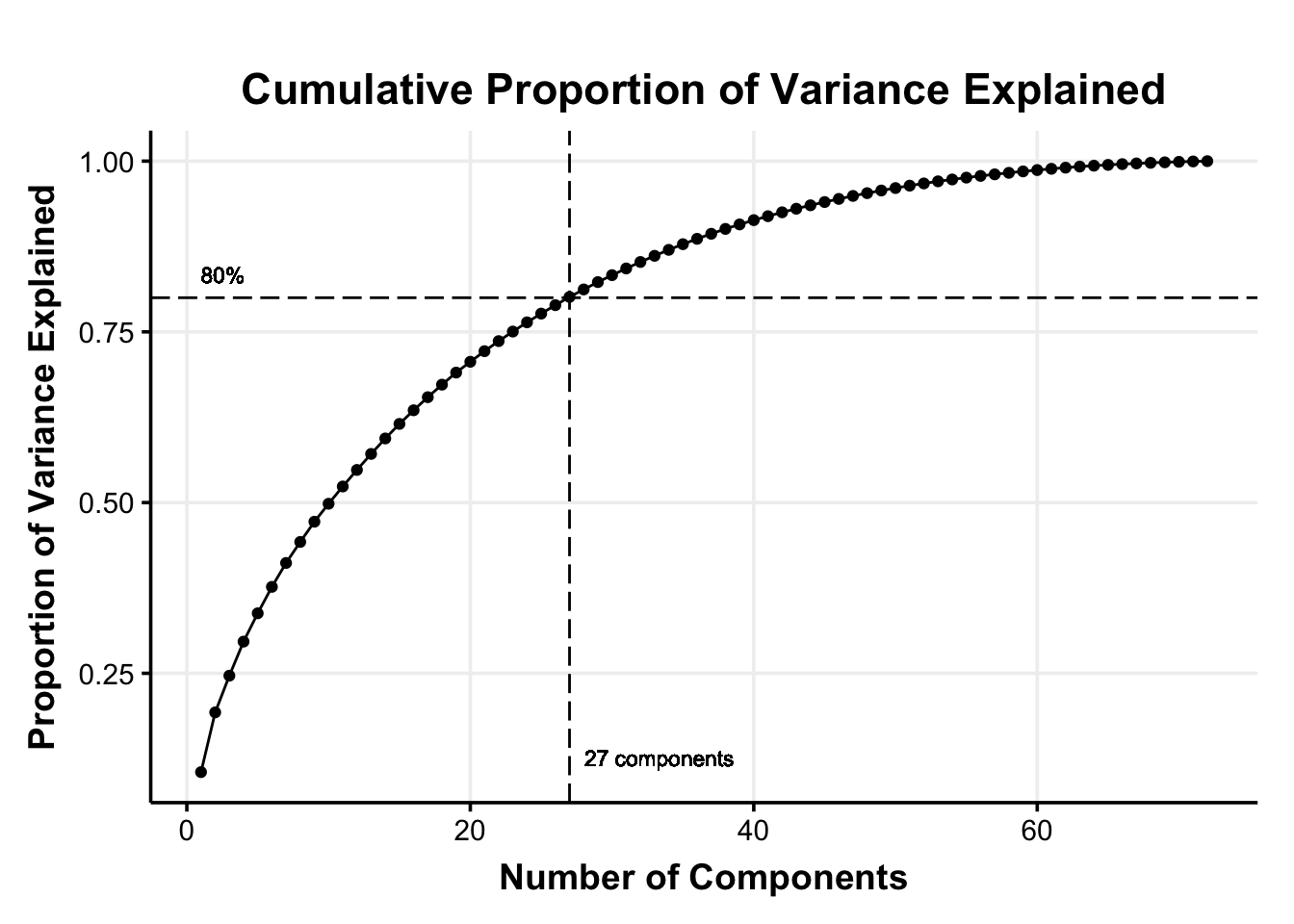
We can then also get a slightly better of an understanding of how the data is distributed by visualizing the features and the participants within the lower dimensional space. We here chose the first three principal components to allow for human undestandable dimensionality.
plot1 <- plot_ly(
  res.pca$rotation %>% as.data.frame,
  x = ~ PC1,
  y = ~ PC2,
  z = ~ PC3,
  size = 2,
  type = 'scatter3d',
  mode = 'markers',
  text = ~ paste('Variable:', rownames(res.pca$rotation))
) %>%
  layout(title = 'Variables in reduced space')
plot2 <- plot_ly(
  res.pca$x %>% as.data.frame,
  x = ~ PC1,
  y = ~ PC2,
  z = ~ PC3,
  size = 2,
  type = 'scatter3d',
  mode = 'markers',
  text = ~ paste('Participant:', rownames(res.pca$x))
) %>%
  layout(title = 'Participants in reduced space')

# Display side by side using htmltools
div(
  style = "display: flex; justify-content: space-between;",
  list(
    div(plot1, style = "width: 50%;"),
    div(plot2, style = "width: 50%;")
  )
)
Save Principal Component Scores
For the extracted principal components we save the 27 principal component scores for each participant (i.e., the participants’ coordinates in the reduced dimensional space; PC-scores) in the pca_scores data frame.
It is important to note that we do not standardize the principal component scores again before adding them into the clustering algorithm. With the PCs the differences in variances are crucial to the dimensionality reduction and standardizing the PC-scores would remove this information.
pca_scores %>%
  summarize_all(sd) %>%
  pivot_longer(everything(), names_to = "PC", values_to = "sd") %>%
  ggplot(., aes(x=reorder(PC, sd), y=sd, label=sd)) +
  geom_bar(stat='identity', width=.5) +
  coord_flip() +
  labs(
    x = "Principal Component",
    y = "Standard Deviation",
    title = "Standard Deviation of each Principal Component"
  ) +
  theme_Publication()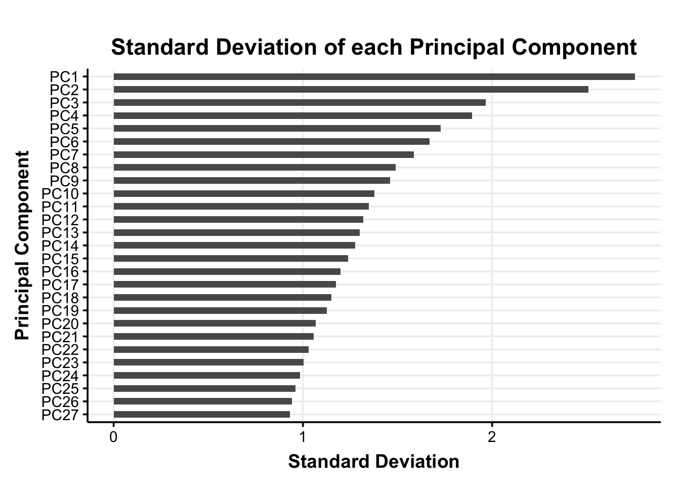
With the reduced variable space of the PC-scores we can now move on to the clustering of the data.