5. Cluster Evaluation

Now that the participants have been assigned to their respective clusters based on the similarity of their time series features, the final evaluation step includes two main elements, (1) evaluating the performance of the clustering analyses to choose an optimal solution and (2) interpreting the extracted clusters conceptually.

Performance

In the performance evaluation step, we are mainly concerned with finding the optimal clustering solution. In the previous step, we extracted 9 possible solutions that might all be good at separating the participants. We thus have to evaluate and compare the performance of each solution. In practical terms, performance evaluation often means assessing the accuracy, stability, and separation or purity of the clustering (Keogh & Kasetty, 2003). In our own illustration example, we used the cluster.stats() function from the fpc package, which calculates a wide variety of internal cluster validity statistics for each of the extracted clustering solutions.

kmeans_performance <- list()
for (i in 2:10) {
  kmeans_performance[[i - 1]] <-
    fpc::cluster.stats(
      d = dist(pca_scores),
      clustering = kmeans_results[[i - 1]]$cluster,
      G2 = TRUE,
      G3 = TRUE,
      aggregateonly = TRUE
    ) %>% unlist
}
df_kmeans_performance <-
  data.frame(Reduce(rbind, kmeans_performance))

kmeans_metrics_names <- c(
  "n" = "number of cases", 
  "cluster.number" = "number of points", 
  "min.cluster.size" = "size of smallest cluster", 
  "noisen" = "number of noise points", # Not relevant for kmeans 
  "average.between" = "average distance between clusters", 
  "average.within" = "average distance within clusters", # (reweighted so that every observation, rather than every distance, has the same weight)
  "max.diameter" = "maximum cluster diameter",
  "min.separation" = "minimum cluster separation", 
  "ave.within.cluster.ss" = "within clusters sum of squares", # generalisation
  "avg.silwidth" = "average silhouette width", 
  "g2" = "Goodman Kruskal's Gamma coefficient", # See Milligan and Cooper (1985), Gordon (1999, p. 62). 
  "g3" = "G3 coefficient", # See Gordon (1999, p. 62)
  "pearsongamma" = "Normalized gamma", # correlation between distances and a 0-1-vector where 0 means same cluster, 1 means different clusters. see Halkidi et al. (2001)
  "dunn" = "Dunn index", # minimum separation / maximum diameter, Dunn index, see Halkidi et al. (2002).
  "dunn2" = "Dunn index 2", # minimum average dissimilarity between two cluster / maximum average within cluster dissimilarity, another version of the family of Dunn indexes
  "entropy" = "entropy of distribution of cluster memberships", # see Meila(2007)
  "wb.ratio" = "average within / average between", 
  "ch" = "Calinski and Harabasz index", # (Calinski and Harabasz 1974, optimal in Milligan and Cooper 1985; generalised for dissimilarites in Hennig and Liao 2013)
  "widestgap" = "widest within-cluster gap", 
  "sindex" = "separation index"
)

df_kmeans_performance %>%
  kbl(.,
      escape = FALSE,
      booktabs = TRUE,
      align = "c",
      digits = 2,
      row.names = FALSE,
      col.names = kmeans_metrics_names) %>%
  kable_classic(
    full_width = F,
    lightable_options = "hover",
    html_font = "Cambria"
  ) %>%
  scroll_box(width = "100%")

Table 1: Cluster Performance for k = 2–10
number of cases	number of points	size of smallest cluster	average distance between clusters	average distance within clusters	maximum cluster diameter	minimum cluster separation	within clusters sum of squares	average silhouette width	Goodman Kruskal's Gamma coefficient	G3 coefficient	Normalized gamma	Dunn index	Dunn index 2	entropy of distribution of cluster memberships	average within / average between	Calinski and Harabasz index	widest within-cluster gap	separation index
156	2	76	10.98	9.98	19.77	4.70	51.80	0.09	0.26	0.36	0.21	0.24	1.10	0.69	0.91	16.38	12.48	5.54
156	3	41	10.91	9.70	18.93	4.89	48.47	0.08	0.32	0.31	0.26	0.26	1.04	1.08	0.89	13.96	12.48	5.40
156	4	21	10.92	9.54	18.54	5.15	46.58	0.08	0.40	0.26	0.30	0.28	0.93	1.32	0.87	11.68	12.48	5.51
156	5	5	10.95	9.44	18.00	4.89	45.05	0.08	0.45	0.24	0.33	0.27	0.80	1.41	0.86	10.28	13.34	5.39
156	6	5	10.80	9.32	18.00	4.69	43.67	0.06	0.44	0.24	0.28	0.26	0.77	1.68	0.86	9.37	13.34	5.26
156	7	5	10.77	9.23	18.00	5.03	42.48	0.06	0.45	0.23	0.28	0.28	0.74	1.84	0.86	8.67	13.34	5.31
156	8	5	10.74	9.12	18.00	4.69	41.31	0.05	0.48	0.22	0.27	0.26	0.73	1.99	0.85	8.19	13.34	5.15
156	9	5	10.71	9.04	18.00	4.69	40.31	0.05	0.49	0.22	0.26	0.26	0.74	2.12	0.84	7.75	13.34	5.09
156	10	2	10.74	9.04	18.00	4.69	39.35	0.05	0.51	0.21	0.29	0.26	0.63	2.07	0.84	7.40	13.92	5.09

With real-world data no single evaluation measure is likely perfect, and different measures may produce different results depending on the characteristics of the data and the research question being addressed (Kittler et al., 1998). We found that across most indices, the analysis with \(k=2\) clusters performed the best (see Table 1).

Visual Illustration

Two commonly reported performance measures showed this visually as well. The first statistic is the total within-cluster sum of square \(WCSS\). While the within-cluster variation will naturally decrease with (more) smaller clusters, we observed that the decrease in \(WCSS\) was largest until \(k=2\) after which the decrease was much smaller. This method is also sometimes referred to as the ‘elbow method’ (Syakur et al., 2018).

fviz_nbclust(pca_scores, kmeans, method = "wss") +
  geom_vline(xintercept = 2, linetype = 2)+
  labs(subtitle = "Performance Metric: Elbow method") +
  theme_Publication()

A second, commonly used measure is the average silhouette score. This statistic measures the degree to which each time feature data point is similar to other points within the same cluster, compared to points in other clusters (Rousseeuw, 1987). In our case, the \(k=2\) solution maximized the silhouette coefficient (\(s_2=\) 0.09).

fviz_nbclust(pca_scores, kmeans, method = "silhouette")+
  labs(subtitle = "Performance Metric: Silhouette method") +
  theme_Publication()

Best-performing Solution

We thus, save the \(k=2\) solution as the final model kmeans_final.

set.seed(12345)
kmeans_final <- kmeans(pca_scores, centers = 2, nstart = 100)
kmeans_final$cluster

  1   2   3   4   5   6   7   8   9  10  11  12  13  14  15  16  17  18  20  21 
  2   2   2   1   2   2   2   2   2   1   2   2   2   2   2   2   1   1   1   2 
 22  23  24  25  26  27  28  29  30  31  32  33  34  35  36  37  38  39  40  41 
  1   2   2   1   2   1   1   2   2   1   1   1   1   1   2   2   1   1   1   2 
 42  43  44  45  46  47  48  49  50  51  52  53  54  55  56  57  58  59  60  61 
  1   1   1   2   2   1   2   2   2   1   2   1   1   1   2   2   1   2   2   2 
 62  63  64  65  66  67  68  69  70  71  72  73  74  75  76  77  78  79  80  81 
  2   2   1   1   2   2   1   2   1   1   1   1   2   1   2   1   2   2   2   1 
 82  83  84  85  86  87  88  89  90  91  92  93  94  95  96  97  98  99 100 101 
  1   2   1   1   1   1   1   2   1   2   2   1   1   2   2   1   1   2   1   2 
102 103 104 105 106 107 108 109 110 111 112 113 114 115 116 117 118 119 120 121 
  1   1   1   1   2   1   2   1   2   2   1   2   2   1   1   2   2   2   2   2 
122 123 124 125 126 127 128 129 130 131 132 133 134 135 136 137 138 139 140 141 
  2   1   2   1   1   1   1   1   1   1   2   2   2   2   1   2   2   1   2   2 
142 143 144 145 146 147 148 149 150 151 152 153 154 155 156 157 
  1   1   1   2   1   2   2   1   2   1   2   1   2   1   1   2

saveRDS(kmeans_final, file = "data/kmeans_final.Rds")

We can then use the cluster assignments to visualize the two clusters. This is commonly done using a projection method where the group separation is visualized on a two-dimensional pane. This is not ideal (because the clustering takes a multi-dimensional space into account), but can give a first indivation of the cluster separation.

# label: visualize the cluster assignment

fviz_cluster(kmeans_final, geom = "point", data = z_data, ggtheme = theme_Publication())

Interpretation

The interpretation of feature-based time series clustering in psychology involves understanding the meaning and implications of the obtained clusters. In order to make sense of the clustering results, we here focus on three general aspects of the results (Kaufman & Rousseeuw, 1990). (1) Assessing differences between the clusters in the original time series features, (2) comparing the clusters based on prototype developments, (3) comparing the clusters based on between-person differences that were not included in the initial clustering.

TS Feature Comparison

We first inspect the clusters based on the average values of meaningful features. To do so, we merge the cluster assignments from the kmeans_final object back to the original set of standardized time series features z_data (same as scaled_data earlier). We then are able to group the features by the clusters and calculate average feature values for each cluster. We also pivot the dataframe into long format for easier visualizations, separate the variable and the feature identifiers, and add more descriptive labels for the visualizations.

# calculate number of removed datapoints
missingness_ooc_id <- full_join(
  featData %>%
    mutate(uid = paste(study, PID, sep = "_")) %>%
    group_by(uid, ID) %>%
    summarise(n_feature = n()) %>%
    ungroup(),
  dt_raw %>%
    mutate(uid = paste(study, PID, sep = "_")) %>%
    group_by(uid) %>%
    summarise(n_raw = n()) %>%
    ungroup(),
  by = "uid"
) %>%
  mutate(
    n_rm = n_raw - n_feature
  ) %>%
  filter(
    !is.na(ID)
  ) %>%
  mutate(nrm_z = scale(n_rm)) %>%
  select(ID, nrm_z)
discrimination_ooc_id <- featData %>% 
  select(ID, EvDayDiscr.post) %>% 
  distinct(ID, EvDayDiscr.post, .keep_all = TRUE) %>%
  mutate(EvDayDiscr.post_z = scale(EvDayDiscr.post, scale = TRUE)) %>%
  replace_na(list(EvDayDiscr.post_z = NA)) %>%
  select(
    ID,
    EvDayDiscr.post_z
  )

featCluster <- data.frame(ID = as.numeric(names(kmeans_final$cluster)), 
                            cluster = kmeans_final$cluster) %>%
  left_join(z_data, by = "ID") %>%
  left_join(discrimination_ooc_id, by = "ID") %>% 
  left_join(missingness_ooc_id, by = "ID") %>%
  select(-ID) %>%
  group_by(cluster) %>%
  summarise(across(everything(), list(mean = mean), na.rm=TRUE)) %>%
  ungroup %>% 
  select(-starts_with("ID")) %>%
  pivot_longer(
    cols = -c(cluster),
    names_to = c("variable", ".value"),
    names_pattern = "(.*)_(.*)"
  ) %>% 
  mutate(
    nam = variable,
    variable = gsub("\\_.*", "", nam),
    feature = gsub("^.*?\\_", "", nam)
  ) %>% 
  mutate(feature = ifelse(feature == "z", "mean", feature)) %>%
  left_join(var_meta %>% select(name, label) %>% rbind(c("nrm", "OOC: Measurements removed")), by = c("variable" = "name")) %>%
  select(
    cluster,
    nam,
    variable,
    label,
    feature,
    everything()
  ) %>% 
  mutate(feature = gsub("^n$", "n (within ooc)", feature)) %>% 
  mutate(feature = gsub("^mean$", "between ooc (mean)", feature))

We can then plot the average features and for each variable and flipping the axes allows us to assess the same data once with a focus on the variable (see Figure 1 A) and once with a focus on the features (see Figure 1 B).

# clusterVariableGrid
clusterVariableGrid <- featCluster %>% 
  filter(variable != "EvDayDiscr.post",
         variable != "nrm",
         feature != "n (within ooc)") %>%
  ggplot(., aes(x = feature, y = mean, group = cluster, color = as.factor(cluster))) +
  geom_point() +
  geom_line() +
  scale_colour_manual(values = c("#384B6B", "#E2892B")) + 
  #geom_errorbar(aes(ymin = mean-se, ymax = mean+se), width=.1, position=position_dodge(0.1), size=0.5, alpha=0.4) +
  coord_flip() +
  labs(
    x = "Features",
    y = "Standardized Mean",
    color = "Cluster"
  ) +
  facet_wrap(~ label) +
  theme_Publication()

# clusterFeatureGrid
clusterFeatureGrid <- featCluster %>% 
  ggplot(., aes(x = reorder(label, as.numeric(!label %in% c("OOC: Discrimination", "OOC: Measurements removed"))), y = mean, group = cluster, color = as.factor(cluster))) +
  geom_point() +
  geom_line() +
  #geom_ribbon(aes(ymin = mean-se, ymax = mean+se), alpha = 0.2) +
  #geom_errorbar(aes(ymin = mean-se, ymax = mean+se), width=.1, position=position_dodge(0.1), size=0.5, alpha=0.4) +
  scale_colour_manual(values = c("#384B6B", "#E2892B")) + 
  coord_flip() +
  labs(
    x = "Variable",
    y = "Standardized Mean",
    color = "Cluster"
  ) +
  facet_wrap(~ factor(feature, levels = unique(featCluster$feature)), ncol=4) +
  theme_Publication()

clusterFeatVarComb <- ggpubr::ggarrange(
  clusterVariableGrid + theme(axis.title.x = element_blank()),
  clusterFeatureGrid,
  ncol = 1,
  labels = c("(A) Variable Focus", "(B) Feature Focus"),
  common.legend = TRUE,
  legend = "bottom",
  align = "v"
) 
ggsave("../Figures/clusterFeatVarComb_tutorial.pdf", clusterFeatVarComb, width = 12, height = 12)
clusterFeatVarComb

Figure 1: Cluster comparison by feature and variable. Note that n and discrimination are out of cluster variables.

We discuss the individual differences and their theoretical relevance as part of the main manuscript. However, in terms of methodological insight, we find variables and features that distinguish the clusters better than others and a combination of variables and features lets us explore meaningful group differences in more detail. In our case, we see that the central tendency, variability, and linear trend are best at distinguishing a group with mainly positive experiences (cluster 1) from a group with a more negative experience (cluster 2). We also see that our clusters line up with the past literature on the importance of focusing on simpler and more meaningful statistics (Bringmann & Eronen, 2018; Eronen & Bringmann, 2021).

Average Time Series

In the second step, we look at the prototypical trajectories of the clusters. For k-means clustering it is often recommended to use the average over time of the responses within the cluster (Niennattrakul & Ratanamahatana, 2007). We visualize the cluster-specific time point averages (see Figure 2 A) as well as an average spline per cluster (see Figure 2 A).

rawCluster <- data.frame(ID = as.numeric(names(kmeans_final$cluster)), 
                            cluster = kmeans_final$cluster) %>%
  left_join(raw_data, by = "ID") %>%
  select(
    ID,
    TIDnum,
    cluster,
    everything()
  ) %>%
  reshape2::melt(id.vars = c("cluster", "ID", "TIDnum")) %>% 
  filter(
    !variable %in% c("PID", "study", "date", "week", "TID", "EvDayDiscr.post"),
    !is.na(value)
  ) %>%
  left_join(var_meta %>% select(name, label), by = c("variable" = "name")) %>%
  mutate(value = as.numeric(value))

clusterTS <- rawCluster %>% 
  ggplot(., aes(x=TIDnum, y=as.numeric(value), group=cluster, color=as.factor(cluster))) +
  geom_line(aes(x=TIDnum, y=as.numeric(value), group=ID, color=as.factor(cluster)), alpha=0.05) +
  stat_summary(fun=mean, geom="line") +
  scale_colour_manual(values = c("#384B6B", "#E2892B")) + 
  facet_wrap(. ~ label) +
  labs(
    x = "Time ID",
    y = "Response (Mean Cluster Response Bold)",
    color = "Cluster"
  ) +
  theme_Publication() 

clusterTSTrend <- rawCluster %>% 
  ggplot(., aes(x=TIDnum, y=value, group=cluster, color=as.factor(cluster))) +
  geom_line(stat="smooth", method = "gam", aes(group=ID, color=as.factor(cluster)), se = FALSE, alpha=0.1) +
  geom_smooth(aes(group=cluster), method = "gam", se = FALSE) +
  scale_colour_manual(values = c("#384B6B", "#E2892B")) + 
  facet_wrap(~ label) +
  scale_y_continuous(limits = c(0, 100)) +
  labs(
    x = "Time ID",
    y = "Response (Mean Cluster Response Bold)",
    color = "Cluster"
  ) +
  theme_Publication()

ggpubr::ggarrange(
  clusterTS + theme(axis.title.x = element_blank()),
  clusterTSTrend,
  ncol = 1,
  labels = c("(A) Timepoint Means", "(B) Spline Trends"),
  common.legend = TRUE,
  legend = "bottom"
)

Figure 2: Average cluster trajectories (using LM and GAM)

While we discuss the interpretations in more detail in the manuscript, the average cluster trajectories offer clearer insights into the mean differences, the variances, as well as the trends over time.

(Out-of-)Cluster Comparison

Finally, we can also assess the clusters across other individual difference variables (Monden et al., 2022). This out-of-feature comparison allows us to check for data artifacts, as well as check whether the developmental clusters are associated with important social markers and individual differences.

To illustrate artifact checks, we added the number of ESM measurements into the comparison and find that the participants in the deterioration cluster (cluster 2) on average completed slightly more ESM surveys in general and reported on more intergroup interactions in particular (see \(n\) in Figure 1 B). This difference in the reported number of interactions might indicate either a clustering artifact or a meaningful difference. The higher average number of interactions in cluster 2 could, for example, indicate a clustering artifact if variances are substantially larger due to the larger samples (e.g., restriction of range in the smaller sample; Kogan et al. (2006)). In our case, this seems less likely because one out of four variables did not differ in terms of the MAD (i.e., our selected measurement of the time series variance; see plot selection below).

# ESM features
raw_feat_clust <-
  data.frame(ID = as.numeric(names(kmeans_final$cluster)),
             cluster = kmeans_final$cluster) %>%
  left_join(z_data, by = "ID")

concepts_and_feature <- str_match(colnames(raw_feat_clust), "(.*)_(.*)")
concepts <- as.character(na.omit(unique(concepts_and_feature[, 2])))
ts_features <- as.character(na.omit(unique(concepts_and_feature[, 3])))

results <- run_all_tests(
  df = raw_feat_clust,
  cluster_var = "cluster",
  ts_features = ts_features,
  concepts = concepts
)

results_df <- convert_test_to_dataframe(
  results = results,
  ts_features = ts_features, 
  concept = concepts
)


# validation features
missingness_ooc <- full_join(
  featData %>%
    mutate(uid = paste(study, PID, sep = "_")) %>%
    group_by(uid, ID) %>%
    summarise(n_feature = n()) %>%
    ungroup(),
  dt_raw %>%
    mutate(uid = paste(study, PID, sep = "_")) %>%
    group_by(uid) %>%
    summarise(n_raw = n()) %>%
    ungroup(),
  by = "uid"
) %>%
  mutate(
    n_rm = n_raw - n_feature
  ) %>%
  filter(
    !is.na(ID)
  ) %>%
  select(ID, n_rm) %>%
  mutate(n_rm_z = scale(n_rm)) %>%
  left_join(data.frame(ID = as.numeric(names(kmeans_final$cluster)),
             cluster = kmeans_final$cluster), by = "ID")
t_missingness <- t.test(
  missingness_ooc$n_rm_z[missingness_ooc$cluster == 1],
  missingness_ooc$n_rm_z[missingness_ooc$cluster == 2],
  na.action = na.omit
)

discrimination_ooc <-
  featData %>% 
  select(ID, EvDayDiscr.post) %>% 
  distinct(ID, EvDayDiscr.post, .keep_all = TRUE) %>%
  mutate(EvDayDiscr.post_z = scale(EvDayDiscr.post, scale = TRUE)) %>%
  replace_na(list(EvDayDiscr.post_z = NA)) %>%
  select(
    ID,
    EvDayDiscr.post_z
  ) %>%
  left_join(data.frame(ID = as.numeric(names(kmeans_final$cluster)),
             cluster = kmeans_final$cluster), by = "ID")

t_discrimination <- t.test(
  discrimination_ooc$EvDayDiscr.post_z[discrimination_ooc$cluster == 1],
  discrimination_ooc$EvDayDiscr.post_z[discrimination_ooc$cluster == 2],
  na.action = na.omit
)

results_df <- rbind(
  results_df,
  data.frame(
    concept = c("EvDayDiscr.post", "missingness"),
    feature = c("mean", "mean"),
    difference = c(t_discrimination$estimate[1] - t_discrimination$estimate[2], t_missingness$estimate[1] - t_missingness$estimate[2]),
    t_value = c(t_discrimination$statistic, t_missingness$statistic),
    df = c(t_discrimination$parameter, t_missingness$parameter),
    p_value = c(t_discrimination$p.value, t_missingness$p.value),
    lwr = c(t_discrimination$conf.int[1], t_missingness$conf.int[1]),
    upr = c(t_discrimination$conf.int[2], t_missingness$conf.int[2])
  )
) %>%
  annotate_significance(., 
                        variableLab = var_meta %>% select(name, label), 
                        join_by = c('concept' = 'name'))

results_df[results_df$concept=="missingness",colnames(results_df)=="label"] <- "Missingness (N removed)"

feature_plot_list <- generate_feature_plots(results_df)

At the same time, however, the difference in the number of experienced interactions might also indicate a meaningful difference, where the deteriorating cluster (cluster 2) on average reported more outgroup interactions (difference = 1.03, t(150.83) = 7.50, p < .001, 95%CI [0.76, 1.30]), but these interactions were less voluntary (difference = -1.04, t(108.89) = -7.71, p < .001, 95%CI [-1.31, -0.77]), less meaningful (difference = -1.00, t(136.40) = -7.16, p < .001, 95%CI [-1.28, -0.73]), and less positive (difference = -1.38, t(152.31) = -11.94, p < .001, 95%CI [-1.61, -1.15]).

To underscore the value of examining out-of-feature individual variations, we also contrasted the two samples based on the participants’ self-reported experiences of discrimination in the Netherlands, captured during the post-measurement phase. Upon analyzing the group differences, it was evident that those in the deteriorating cluster (cluster 2) indicated notably elevated instances of daily discrimination (difference = -0.40, t(151.71) = -2.56, p = 0.011, 95%CI [-0.71, -0.09]; also see Figure 1 B). In short, both intensive longitudinal measurement (e.g., the sum of specific ESM measurements) and cross-sectional variables (e.g., general discrimination differences) that were not included in the original clustering step can be leveraged to delve deeper into understanding cluster disparities.

References

Bringmann, L. F., & Eronen, M. I. (2018). Don’t blame the model: Reconsidering the network approach to psychopathology. Psychological Review, 125(4), 606–615. https://doi.org/10.1037/rev0000108

Eronen, M. I., & Bringmann, L. F. (2021). The Theory Crisis in Psychology: How to Move Forward. 779–788. https://doi.org/10.1177/1745691620970586

Kaufman, L., & Rousseeuw, P. J. (Eds.). (1990). Finding Groups in Data. John Wiley & Sons, Inc. https://doi.org/10.1002/9780470316801

Keogh, E., & Kasetty, S. (2003). On the Need for Time Series Data Mining Benchmarks: A Survey and Empirical Demonstration. Data Mining and Knowledge Discovery, 7(4), 349–371. https://doi.org/10.1023/A:1024988512476

Kittler, J., Hatef, M., Duin, R. P. W., & Matas, J. (1998). On combining classifiers. IEEE Transactions on Pattern Analysis and Machine Intelligence, 20(3), 226–239. https://doi.org/10.1109/34.667881

Kogan, J., Nicholas, C. K., & Teboulle, M. (Eds.). (2006). Grouping multidimensional data: Recent advances in clustering. Springer.

Monden, R., Rosmalen, J. G. M., Wardenaar, K. J., & Creed, F. (2022). Predictors of new onsets of irritable bowel syndrome, chronic fatigue syndrome and fibromyalgia: The lifelines study. Psychological Medicine, 52(1), 112–120. https://doi.org/10.1017/S0033291720001774

Niennattrakul, V., & Ratanamahatana, C. A. (2007). Inaccuracies of Shape Averaging Method Using Dynamic Time Warping for Time Series Data. In D. Hutchison, T. Kanade, J. Kittler, J. M. Kleinberg, F. Mattern, J. C. Mitchell, M. Naor, O. Nierstrasz, C. P. Rangan, B. Steffen, M. Sudan, D. Terzopoulos, D. Tygar, M. Y. Vardi, G. Weikum, Y. Shi, G. D. van Albada, J. Dongarra, & P. M. A. Sloot (Eds.), Computational Science – ICCS 2007 (Vol. 4487, pp. 513–520). Springer Berlin Heidelberg. https://doi.org/10.1007/978-3-540-72584-8_68

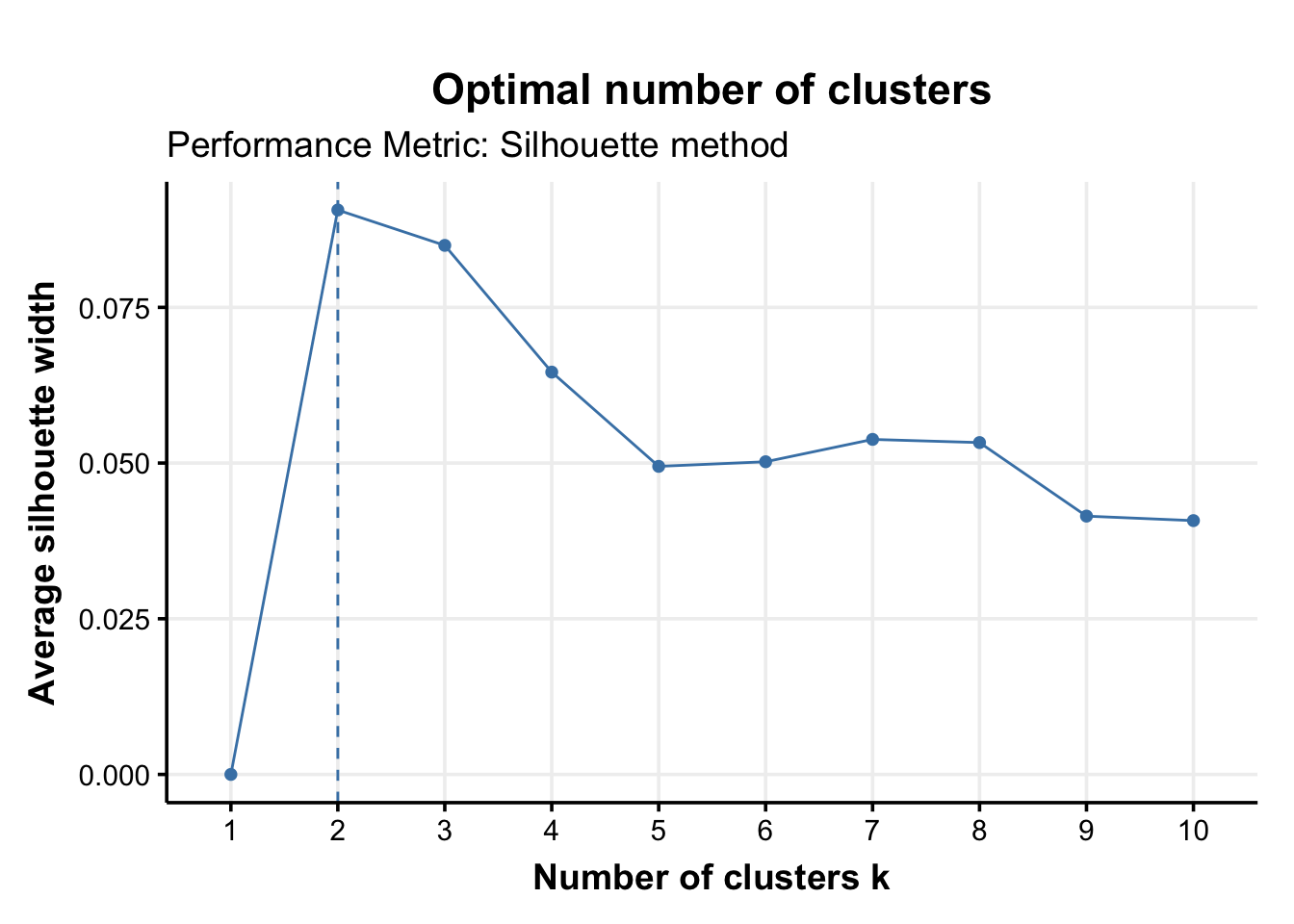
Rousseeuw, P. J. (1987). Silhouettes: A graphical aid to the interpretation and validation of cluster analysis. Journal of Computational and Applied Mathematics, 20, 53–65. https://doi.org/10.1016/0377-0427(87)90125-7

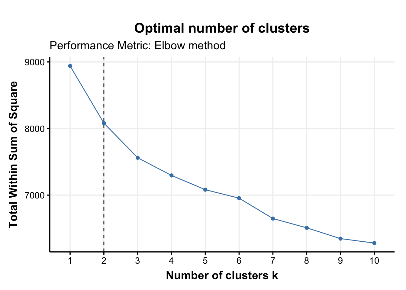
Syakur, M. A., Khotimah, B. K., Rochman, E. M. S., & Satoto, B. D. (2018). Integration K-Means Clustering Method and Elbow Method For Identification of The Best Customer Profile Cluster. IOP Conference Series: Materials Science and Engineering, 336, 012017. https://doi.org/10.1088/1757-899X/336/1/012017