6. Validation Analyses

To further understand our cluster solution and ensure the validity of our results, we ran a number of validation analyses. Within these additional analyses, we assess a single cluster solution, the impact of the missingness handling as well as an alternative analysis with a reduced feature set focusing on non-dynamic features. As an additional resource, we also developed an interactive web application to try out different method and parameter options.

Single Cluster Solution

To ensure that the clustering is necessary in the first place, we also compare the performance to a single cluster solution (i.e., a single centroid). The comparison to this \(k=1\) solution is slightly different because metrics like the between cluster separation are not available. Nonetheless, comparing the within-cluster sums of squares and the explained variance, we find that two clusters indeed are outperforming a single cluster solution.

library(cluster)

numeric_data <- scaled_pc[, sapply(scaled_pc, is.numeric)]

# also calculate k=1 solution
kmeans_one_cluster <- kmeans(numeric_data, centers = 1, nstart = 25)
kmeans_two_clusters <- kmeans(numeric_data, centers = 2, nstart = 25)

# Compare the total within-cluster sum of squares
total_withinss_one_cluster <- kmeans_one_cluster$tot.withinss
total_withinss_two_clusters <- kmeans_two_clusters$tot.withinss


# Calculate the total sum of squares
total_ss <- sum(sapply(numeric_data, function(x) sum((x - mean(x))^2)))
var_explained_one_cluster <- 1 - (total_withinss_one_cluster / total_ss)
var_explained_two_clusters <- 1 - (total_withinss_two_clusters / total_ss)

# create table output
singleClusterPerf <- data.frame(
  Clusters = c("One Cluster", "Two Clusters"),
  TotalWithinSS = c(total_withinss_one_cluster, total_withinss_two_clusters),
  VarianceExplained = c(var_explained_one_cluster, var_explained_two_clusters)
)
singleClusterPerf$VarianceExplained <-
  ifelse(
    singleClusterPerf$VarianceExplained < 0.001,
    "<.001",
    as.character(round(singleClusterPerf$VarianceExplained, 3))
  )
singleClusterPerfNames <- c("Cluster Count", "Total Within-Cluster SS", "Variance Explained")
singleClusterPerf %>%
  kbl(.,
      escape = TRUE,
      booktabs = TRUE,
      align = c("l", "c", "c"),
      digits = 3,
      row.names = FALSE,
      col.names = singleClusterPerfNames,
      caption = "K-Means Single Cluster Performance Comparison") %>%
  kable_classic(
    full_width = FALSE,
    lightable_options = "hover",
    html_font = "Cambria"
  )

K-Means Single Cluster Performance Comparison

Cluster Count	Total Within-Cluster SS	Variance Explained
One Cluster	8940.213	<.001
Two Clusters	8080.674	0.096

Missingness Handling

In our illustration data set, the studies differed substantially in the maximum length of participation (\(max(t_{S1})\) = 63, \(max(t_{S2})\) = 69, \(max(t_{S3})\) = 155). To make the three studies comparable in participation and time frames, we iteratively removed all measurement occasions and participants that had more than 45% missingness in the main text. While this procedure works well for users who wish to use the clustering in combination with other parametric models, the 45% threshold might be too conservative if the analysis stands on its own. We here show how the results would have differed if the missingness threshold is set more liberally.

Sample Extraction

We now run the cleanM function for the completeness thresholds of 0%, 5%, 10%, 15%, 20%, 25%, 30%, 35%, 40%, 45%, 50%, as well as the original 55% (i.e., allowing up to 100% missingness). The non-conforming rows and colums are again sequentially remove staring with the row or column with the most missing data until only rows and columns remain that fit the threshold. The resulting missingess information and reduced datasets are stores in a new list called missingness_samples.

source("scripts/cleanM.R")

# Function to prepare availability data for a given study
prepareAvailabilityData <- function(dt_raw, study_id) {
  dtAvailability <- dt_raw %>%
    filter(study == study_id) %>%
    select(PID, TIDnum) %>%
    arrange(PID, TIDnum) %>%
    mutate(data = 1)
  dtAvailability <- reshape::cast(dtAvailability, PID ~ TIDnum, value = "data", fun.aggregate = length) %>%
    select(-PID) %>%
    mutate_all(function(x) ifelse(x > 1, 1, x))
  return(dtAvailability)
}

# Function to process data for a given study and threshold
processStudyData <- function(dtAvailability, study_id, threshold) {
  dtRedInfo <- cleanM(M = as.data.frame(dtAvailability), c = threshold)
  PIDout <- gsub("PP_", "", dtRedInfo$rowNamesOut) %>% as.numeric
  TIDInRed <- gsub("t_", "", dtRedInfo$colNamesIn) %>% as.numeric
  
  # Check if TIDInRed has valid numeric values
  if (length(TIDInRed) > 0 && all(!is.na(TIDInRed))) {
    TIDIn <- seq(min(TIDInRed, na.rm = TRUE), max(TIDInRed, na.rm = TRUE), 1)
  } else {
    # Handle the case where TIDInRed is empty or invalid
    TIDIn <- numeric(0)  # An empty numeric vector
  }
  
  dtRed <- dt_raw %>%
    filter(study == study_id) %>%
    filter(
      !PID %in% PIDout,
      TIDnum %in% TIDIn
    ) %>%
    mutate(TIDnum = TIDnum - min(TIDnum, na.rm = TRUE))
  
  return(list(dtRedInfo = dtRedInfo, dtRed = dtRed))
}

# Initialize lists to store results
missingness_samples <- list()

# Define the studies and thresholds
studies <- c("S1", "S2", "S3")
completeness_thresholds <- seq(from = 0, to = 55, by = 5)

# Iterate over studies and thresholds
for (study in studies) {
  dtAvailability <- prepareAvailabilityData(dt_raw, study)
  rownames(dtAvailability) <- paste("PP", 1:nrow(dtAvailability), sep = "_")
  colnames(dtAvailability) <- paste("t", 1:ncol(dtAvailability), sep = "_")
  
  for (threshold in completeness_thresholds) {
    result_key <- paste(study, threshold, sep = "_")
    cat("\n\nSTUDY: ", study, "; THRESHOLD: ", threshold, "\n")
    missingness_samples[[result_key]] <- processStudyData(dtAvailability, study, threshold)
  }
}

This allows us to store all the missingess infomation for each study. From this we can extract the reduced data sets for each threshold and combine them into a single reduced data set per threshold. We also save the compute intensive steps for these validation analyses.

# Initialize a list to store the combined data for each threshold
combined_data <- list()

# Unique thresholds are extracted from the list keys
unique_thresholds <- unique(sub(".*_", "", names(missingness_samples)))

# Loop through each threshold
for (threshold in unique_thresholds) {
  # Initialize an empty list to store data for each study at the current threshold
  study_data_list <- list()
  
  # Loop through each study and extract the corresponding dtRed data
  for (study in c("S1", "S2", "S3")) {
    key <- paste(study, threshold, sep = "_")
    dtRed <- missingness_samples[[key]]$dtRed
    
    # Apply the necessary transformations
    dtRed_transformed <- dtRed %>%
      select(-c("created", "ended")) %>%
      mutate(study = study) # %>%
      # mutate(across(!TID & !study, as.numeric))
    
    # Store the transformed data in the list
    study_data_list[[study]] <- dtRed_transformed
  }
  
  # Combine the data from all three studies for the current threshold
  dtAll <- bind_rows(study_data_list) %>%
    group_by(study, PID) %>%
    mutate(ID = cur_group_id()) %>%
    ungroup %>%
    mutate(date = as.Date(gsub(" .*", "", TID)),
           week = strftime(date, format = "%Y-W%V")) %>%
    select(ID, PID, study, date, week, TIDnum, everything()) %>%
    arrange(ID, TIDnum) %>%
    select_if(~ sum(!is.na(.)) > 1) %>%  # only include variables that have any data
    as.data.frame
  
  # Store the combined data frame in the list
  combined_data[[threshold]] <- dtAll
}

# Save so that we do not have to run this compute intensive step again
saveRDS(combined_data, "data/missingness_thresholds/01_raw_combined/combined_data.rds")

Feature Extraction

With the reduced data sets for each threshold extracted, we can extract the features for each participant within the reduced data sets. The process is exactly the same as for the main analysis just looping over the thresholds in the combined_data list. We store the resulting feature lists in the feature_results elment which keeps all relevant matrices and data.frames for each threshold dataset.

# devtools::install_github("JannisCodes/tsFeatureExtracR")
library(tsFeatureExtracR)

# Define the directory to store the results
base_dir <- "data/missingness_thresholds/02_features"

# Check if the directory exists; if not, create it
if (!dir.exists(base_dir)) {
  dir.create(base_dir, recursive = TRUE)
}

# Initialize a list to store the feature extraction results for each threshold
feature_results <- list()

feature_selection <- c(
  "ar01",
  "edf",
  "lin",
  "mac",
  "mad",
  "median"
)

# Loop through each dataset in combined_data
for (threshold in names(combined_data)) {
  dtAll <- combined_data[[threshold]]

  # Ensure the dataset only contains variables with any data
  featData <- dtAll %>%
    arrange(ID, TIDnum) %>%
    select_if(~ sum(!is.na(.)) > 1) %>% 
    as.data.frame
  
  # Check for duplicates and remove all occurrences
  duplicate_indices <- duplicated(featData[c("ID", "TIDnum")]) | duplicated(featData[c("ID", "TIDnum")], fromLast = TRUE)
  if (any(duplicate_indices)) {
    warning("Duplicate rows based on ID and TIDnum have been found. All instances will be removed.")
    # Remove all instances of duplicates
    featData <- featData[!duplicate_indices, ]
  }
  
  cat("\n\nExtracting Features for threshold: ", threshold, "\n")
  # Extract features for the current threshold dataset
  featFull <- featureExtractor(
    data = featData,
    pid = "ID",
    tid = "TIDnum",
    items = var_meta$name[var_meta$cluster == 1]
  )

  # Filter out unwanted data (e.g., internal test accounts)
  featFull$features <- featFull$features %>%
    filter(ID != 19)

  # Handle missing features
  perc_miss_features <- feature_missing(featFull$features %>% 
                    select(ends_with(feature_selection)), 
                  title = paste("Feature-wise Missingness for threshold:", threshold, "percent"))
  
  cat("Imputing missing features for threshold: ", threshold, "\n")
  # Impute missing features
  featFullImp <- featureImputer(featFull)

  # Store the results
  feature_results[[threshold]] <- list(
    features = featFullImp,
    missingness_plot = perc_miss_features$plt_miss_per_feature
  )
  cat("Added features for threshold: ", threshold, ".\n")
  
  # Save locally 
  features_path <- file.path(base_dir, paste0("features_", threshold, ".rds"))
  missingness_plot_path <- file.path(base_dir, paste0("missingness_plot_", threshold, ".png"))
  
  # Save the feature results
  saveRDS(feature_results[[threshold]]$features, features_path)
  
  # Save the missingness plot
  png(missingness_plot_path)
  print(feature_results[[threshold]]$missingness_plot)
  dev.off()
  cat("Feature results and missingness plots for threshold: ", threshold, " have been saved in", base_dir, "\n")
}

# Save so that we do not have to run this compute intensive step again
saveRDS(feature_results, "data/missingness_thresholds/02_features/features_all.rds")
cat("All feature results have been saved in", base_dir, ". \n\n*Done!*")

Run Analyses

We run the same set of analyses (i.e., a PCA and a k-means clustering) for each of the feature sets that we extracted based on the different thresholds. To full automate this process, we again select the principal components to capture 80% of the original variance and we use a number of different performance metrics for different \(k\)s in the k-means analysis to select the \(k\) that is optimal according to the most metrics. We also set a random seed set.seed(12345) for strict reproducibility.

analysis_results <- list()

for (threshold in names(feature_results)) {
  
  # Set seed for reproducibility
  set.seed(12345)
  
  cat("\n\nRunning Analyses for", threshold)
  scaled_data <- feature_results[[threshold]]$features$featuresImpZMat %>%
    select(ends_with(feature_selection)) 
  
  # Check for and handle NA values
  if (anyNA(scaled_data)) {
    warning(paste("NA values found in scaled data for threshold", threshold))
    next  # Skip this iteration if NA values are found
  }
  
  # PCA 
  res.pca <- prcomp(scaled_data, scale. = FALSE)
  cutoff_percentage <- 0.8
  pca_cutoff <- min(which(cumsum(summary(res.pca)[["importance"]]['Proportion of Variance',]) >= cutoff_percentage))
  pca_scores <- as.data.frame(res.pca$x[,1:pca_cutoff])
  
  # kmeans with NbClust to find the best number of clusters
  kmeans_performance <- NbClust::NbClust(data = pca_scores, diss = NULL, distance = "euclidean",
                                  min.nc = 2, max.nc = 15, method = "kmeans", index = "all")
  kmeans_best_k <- kmeans_performance$Best.nc["Number_clusters", ] %>%
    as.numeric() %>%
    table() %>%
    which.max() %>%
    names() %>%
    as.numeric()
  kmeans_results <- kmeans(pca_scores, centers = kmeans_best_k, nstart = 100)
  
  analysis_results[[threshold]] <- list(
    pca_scores = pca_scores,
    kmeans_results = kmeans_results
  )
}

# Save so that we do not have to run this compute intensive step again
saveRDS(analysis_results, "data/missingness_thresholds/03_analysis/analysis_results_all.rds")
cat("All analysis results have been saved in", base_dir, ". \n\n*Done!*")

Compare Results

To compare the results from the different missingness thresholds we look at the optimal number of clusters (\(k\)) as well as the similarity of the extracted cluster solutions.

We find that with almost all missingness thresholds the optimal number of k-means clusters is 2. The only exceptions are at the thresholds of 0% = 3, 10% = 5, and 25% = 3 (i.e., 0% threshold = 100% missingness allowed for each).

# Initialize an empty list to store the data frames for each threshold
threshold_dfs <- list()

for (threshold in names(analysis_results)) {
  
  # extract unique ids from data reduction
  red_ids <- combined_data[[threshold]] %>%
    mutate(uid = paste(study, PID, sep = "_")) %>%
    select(ID, uid) %>% 
    distinct() 
  
  # Extract the data frame for the current threshold
  cluster_assignments <- feature_results[[threshold]]$features$features %>%
    select(ID) %>%
    mutate(!!paste("cluster", threshold, sep = "_") := analysis_results[[threshold]]$kmeans_results$cluster)
  
  # join cluster assignments and uids
  df <- red_ids %>%
    full_join(cluster_assignments, by = "ID") %>%
    select(-ID)
  
  # Store the data frame in the list
  threshold_dfs[[threshold]] <- df
}

# Combine all the data frames into a single data frame
threshold_cluster_assignments <- reduce(threshold_dfs, full_join, by = "uid")

# Apply max function to each column, excluding 'uid'
max_values <- apply(threshold_cluster_assignments %>% select(-uid), 2, max, na.rm = TRUE)

# Convert the max values into a data frame
data.frame(k = max_values) %>%
  rownames_to_column("threshold") %>%
  mutate(threshold = paste(gsub("cluster_", "", threshold), "%", sep = ""))%>%
  kbl(.,
      escape = FALSE,
      booktabs = TRUE,
      label = "optimal_k_threshold",
      format = "html",
      digits = 2,
      linesep = "",
      align = c("c", "c"),
      col.names = c("Missingeness Threshold", "Optimal k"),
      caption = "Optimal K based on Missingess Approach") %>%
  kable_classic(
    full_width = FALSE,
    lightable_options = "hover",
    html_font = "Cambria"
  )

Optimal K based on Missingess Approach

Missingeness Threshold	Optimal k
0%	3
5%	2
10%	5
15%	2
20%	2
25%	3
30%	2
35%	2
40%	2
45%	2
50%	2
55%	2

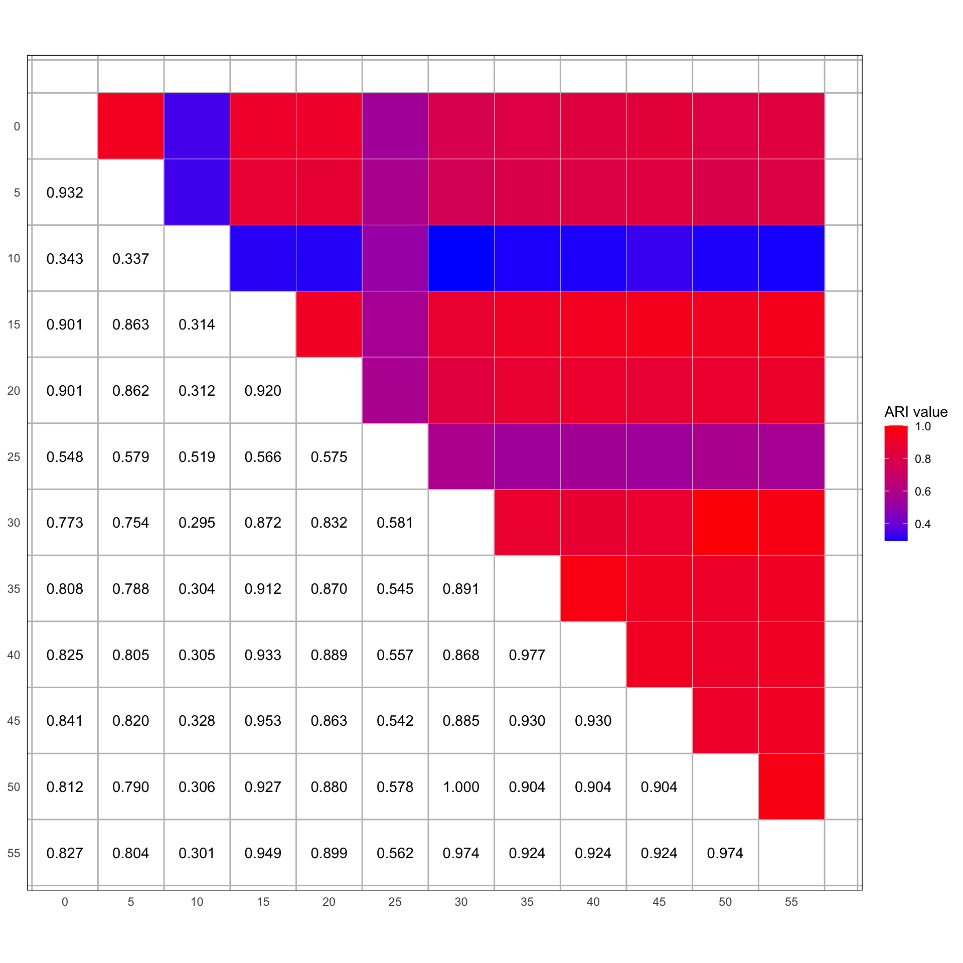
We then compare the clustering results obtained at different thresholds using the Adjusted Rand Index (ARI), which quantifies the similarity between two data clustering assignments. By calculating the ARI for every pair of threshold-based clusterings, we can assess how consistent the cluster assignments are across varying thresholds, even when the number of clusters or their composition changes. This comparison helps us understand the stability of our clustering solution and identify which thresholds yield similar or distinct grouping patterns, providing valuable insights into the robustness of our clustering approach against parameter variations. The ARI is normalized such that -1 indicates perfect disagreement, 0 indicates random (or chance) clustering, and 1 indicates perfect agreement. As a rule of thumb, let us consider that scores close to 0 or negative indicate bad or no similarity (worse than chance), values between 0 and 0.5 reflect reasonable to moderate similarity, scores above 0.5 suggest good similarity, and values close to 1 represent excellent similarity, indicating nearly identical cluster assignments (Hubert & Arabie, 1985).

# Calculate ARI values
library(mclust)  # For ARI calculation

# Initialize a matrix to store the ARI values
n <- length(threshold_dfs)
comparison_matrix <- matrix(NA, n, n, dimnames = list(names(threshold_dfs), names(threshold_dfs)))

# Double loop to compare each pair of thresholds
for (i in 1:(n - 1)) {
  for (j in (i + 1):n) {
    # Extract the cluster assignments for the two thresholds being compared
    threshold_i <- threshold_dfs[[i]]
    threshold_j <- threshold_dfs[[j]]
    
    # Merge the two data frames on uid to find common participants
    merged_df <- merge(threshold_i, threshold_j, by = "uid", all = FALSE)  # all = FALSE ensures only common uids
    
    # Ensure there are no NAs before calculating ARI
    valid_entries <- complete.cases(merged_df)
    merged_df <- merged_df[valid_entries,]
    
    # Check if there are enough common participants to compare
    if (nrow(merged_df) > 1) {
      # Calculate ARI for common participants
      ari_value <- adjustedRandIndex(merged_df[, paste("cluster", names(threshold_dfs)[i], sep = "_")],
                                     merged_df[, paste("cluster", names(threshold_dfs)[j], sep = "_")])
    } else {
      # Not enough data to compare
      ari_value <- NA
    }
    
    # Store the ARI value in the matrix
    comparison_matrix[i, j] <- ari_value
    comparison_matrix[j, i] <- ari_value  # ARI is symmetric
  }
}

# calculate the average ARI for description
avg_ari <- mean(comparison_matrix[upper.tri(comparison_matrix)]) %>%
  format(., digits = 3, nsmall = 3)
remove <- c("0", "10", "25")
avg_ari_k2 <- comparison_matrix[!rownames(comparison_matrix) %in% remove, !colnames(comparison_matrix) %in% remove] %>%
  .[upper.tri(.)] %>% 
  mean() %>%
  format(., digits = 3, nsmall = 3)

# Convert the matrix to a long format suitable for ggplot
comparison_matrix_long <- comparison_matrix %>%
  as.data.frame() %>%
  rownames_to_column("row") %>%
  mutate(row = as.numeric(row)) %>%
  gather(key = "column", value = "value", -row) %>%
  mutate(
    column = as.numeric(column),
    value = as.numeric(format(value, digits = 3, nsmall = 3))
  )

# Create the plot
ggplot(comparison_matrix_long, aes(x = row, y = column, fill = value)) +
  geom_tile(data = subset(comparison_matrix_long, row > column), aes(fill = value), color = "white") +
  scale_fill_gradient(low = "blue", high = "red", na.value = "white", limits = range(comparison_matrix_long$value, na.rm = TRUE), name = "ARI value") +
  geom_text(data = subset(comparison_matrix_long, row < column), aes(label = sprintf("%.3f", as.numeric(value))), color = "black") +
  scale_y_reverse(breaks = seq(0, 55, 5), labels = seq(0, 55, 5)) +
  scale_x_continuous(breaks = seq(0, 55, 5), labels = seq(0, 55, 5)) +
  coord_fixed() +
  theme_minimal() +
  theme(axis.title = element_blank(),
        panel.grid.major = element_blank(),
        panel.grid.minor = element_line(color = "grey", size = 0.5),
        panel.border = element_rect(color = "black", fill = NA))

ARI Comparison Plot

We find that with the exception of when the optimal solution is larger than 2 the cluster similarity is extremely high (see threshold = 10% as an example). In short, the number of clusters seems to be a much bigger decision than the actual cluster assignment itself. At the same time however, the ARIs seem to suggest that the differences in features extracted based on the different missingness thresholds is negligible (as long as the number of clusters is the same). In fact the mean ARI is 0.743 (and the mean ARI for all \(k=2\) is 0.892).

Simplified Model

One question that remains is whether a much simpler model with only central tendency and variance would perform similarly well and would result in a similar separation of the clusters. We here adjust the code we used for the main analysis (just on a smaller feature set). Wherever the code is functionally unchanged from the main analysis we do not rehash it here. If you would like to inspect the full code, you can do this via our OSF and GitHub repositories (referenced in the about page).

Prepare Data

We follow the same data preparation steps as during the main analysis.

feature_selection_full <- c(
  "ar01",
  "edf",
  "lin",
  "mac",
  "mad",
  "median"
)

feature_selection <- c(
  "mad",
  "median"
)

scaled_data_simple <- featFullImp$featuresImpZMat %>% select(ends_with(feature_selection)) 
z_data_simple <- featFullImp$featuresImpZ %>% select("ID", ends_with(feature_selection))

z_data <- featFullImp$featuresImpZ %>% select("ID", ends_with(feature_selection_full))

Run Analyses

Also our analysis steps are identical to the main analysis. We find that in the reduced feature set, \(k=2\) are the most optimal solutions. We extract the k-means cluster assignments for this model.

res.pca_simple <- prcomp(scaled_data_simple, scale. = FALSE)
cutoff_percentage <- 0.8
pca_cutoff_simple <- min(which(cumsum(summary(res.pca_simple)[["importance"]]['Proportion of Variance', ]) >= cutoff_percentage))
pca_scores_simple <- as.data.frame(res.pca_simple$x[, 1:pca_cutoff_simple])

# kmeans with NbClust to find the best number of clusters
kmeans_performance_simple <-
  NbClust::NbClust(
    data = pca_scores_simple,
    diss = NULL,
    distance = "euclidean",
    min.nc = 2,
    max.nc = 15,
    method = "kmeans",
    index = "all"
  )

kmeans_best_k_simple <-
  kmeans_performance_simple$Best.nc["Number_clusters",] %>%
  as.numeric() %>%
  table() %>%
  which.max() %>%
  names() %>%
  as.numeric()

set.seed(42)
kmeans_results_simple <- kmeans(pca_scores_simple, centers = kmeans_best_k_simple, nstart = 100)

Compare Results

We begin by comparing the simpler model to the model from the main analysis in terms of performance and similarity.

Performance

To assess the performance of the clustering algorithm with the parameters you have selected, we display a number performance metrics. These metrics can be divided into ‘general performance’ (looking at separation and cohesion) and ‘cluster structure’ (distribution of points across clusters and the compactness of clusters). We have selected three common metrics for each of the categories. For the general performance we inspect:

Average Silhouette Width

This metric provides a measure of how close each point in one cluster is to points in the neighboring clusters. Higher silhouette width indicates better separation and cohesion.

Calinski and Harabasz Index

This index is a ratio of between-cluster variance to within-cluster variance. Higher values generally indicate clusters are well separated and well defined.

Dunn Index

Measures the ratio of the smallest distance between observations not in the same cluster to the largest intra-cluster distance. Higher values indicate better clustering by maximizing inter-cluster distances while minimizing intra-cluster distances.

For the cluster structure, we display:

Entropy of Distribution of Cluster Memberships

Provides a measure of how evenly data points are spread across the clusters. Lower entropy indicates a more definitive classification of points into clusters.

Minimum Cluster Size

Indicates the size of the smallest cluster. This is useful for identifying if the clustering algorithm is producing any very small clusters, which might be outliers or noise.

Average Distance Within Clusters

This metric offers insight into the compactness of the clusters. Lower values indicate that points within a cluster are closer to each other, suggesting better cluster cohesion.

			General Clustering Performance			Cluster Structure Insight
Analysis Label	number of cases	number of points	average silhouette width	Calinski and Harabasz index	Dunn index	entropy of distribution of cluster memberships	size of smallest cluster	average distance within clusters
main	156	2	0.09	16.38	0.24	0.69	76	9.98
simplified	156	2	0.21	48.38	0.14	0.69	72	5.31

We find that both models perform well across the performance metrics.

Similarity

Similar to the missingness threshold models above, we also look at the Adjusted Rand Index (ARI) to compare the similarity of the models.

We find a relatively high Adjusted Rand Index: \(ARI=\) 0.758 — indicating that the simplified model separates the two clusters in a similar manner.

Full TS Feature Comparison

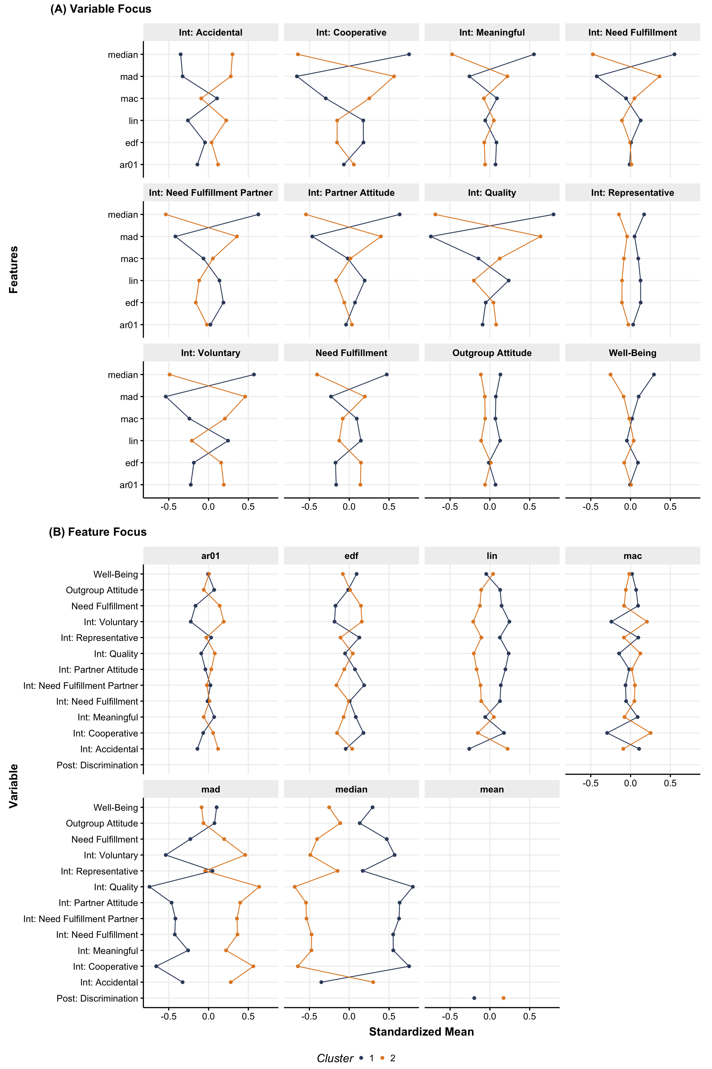
We can then plot the average features and for each variable and flipping the axes allows us to assess the same data once with a focus on the variable (see Figure 1 A) and once with a focus on the features (see Figure 1 B).

Figure 1: Cluster comparison by feature and variable. Note that n and discrimination are out of cluster variables.

As was already indicated by the \(ARI\), the clusters differences look very similar to that of the main analysis, with slightly larger Median and MAD differences but slightly smaller differences in most of the other features (across the variables).

Alternative Models

As a final resource, we have developed a web application offers an interactive dashboard for exploring and understanding time series feature clustering based on the data set of the main analyses. This web application is designed to facilitate the exploration of different clustering algorithms and dimensionality reduction techniques. As the web application accompanies this article, we focus on the time series features from the main analysis data set. The web application is designed to be relevant for several target groups, including researchers, students, or data enthusiasts. The tsFeatureClustR Web App offers a hands-on experience that aims to enhance the understanding of time series data clustering and its underlying processes.

We allow users to try out different combinations of dimensionality reduction algorithms (PCA, t-SNE, Autoencoder, UMAP) and clustering algorithms (k-means, DBSCAN, Hierarchical agglomerative clustering). For each of the methods, we have developed an interface that lets users explore the key parameter settings of the algorithms. To provide an introduction to the diversity of possible combinations, we have pre-calculated the performance of the algorithm combinations for common parameter values (showing users a comparison of up to 18,557 model combinations). On a second panel, readers then have the chance to explore the cluster results based on their own interaction with the different parameters.

If you would like to explore the different alternative models, you can follow the following link:

To the Web App

References

Hubert, L., & Arabie, P. (1985). Comparing partitions. Journal of Classification, 2(1), 193–218. https://doi.org/10.1007/BF01908075